Chapter 3: A tour of risk and performance
- Alpha is the expected value of the idiosyncratic return and epsilon is the noise masking it.
- There's general agreement that accurately forecasting market returns is very difficult or at least not the mandate of a fundamental analyst. A macro investor may have an edge in forecasting the market, but the fundamental one does not have a differentiated view.
- The job of the fundamental investor is to estimate alpha accurately
- The risk manager is job is to estimate beta and identify the correct benchmark
- The error around an alpha estimate is larger than that alpha estimate itself. This is not true for beta. You cannot observe alpha directly and you cannot estimate it from a time series of returns. The fundamental analyst predicts forward looking alphas based on deep research. The ability to combine these alpha forecasts from a variety of sources and process a large number of unstructured data is a competitive advantage of the fundamental investor
- The chapter decomposes alpha(idio) and beta contribution and risks
- What the industry calls “idio”, I refer to as “risk remaining”. Same exact concept.
- If X = market and Y = stock then this identity decomposes the risk:
- Stock variance = Market variance + Idio variance
- Risk remaining or idio is a non-linear function of correlation. As correlation drops, idio explodes. Once R is .86 or lower the idio risk exceeds the market risk!!
[Kris: found this helpful for computing portfolio alpha I’ve covered this all before in https://moontowermeta.com/from-capm-to-hedging/
Var (Y) = * (VarY/VarX) + (1-) * (VarY/VarX)
Note that market variance is
Recall that B = R * ratio of volatility between Y and X
- Shorting SPY to hedge out beta and have absolute return dependent strictly on idio
Chapter 4: An introduction to multi-factor models
- Bar Rosenberg was an academic who started Barra, now MSCI, BGI (acquired by Blackrock), and Axa Rosenberg.
- Since 1981 there has been an explosion of factors explaining equity returns. The methodologies were later extended to other assets like government and corporate credit.
- How are the factors discovered? And where do the betas come from? There are three broad ways to attack the problem.
- The time-series approach, most popular in academia, is often used in conjunction with the fundamental approach. We are surrounded by time-series data: macroeconomic indicators, inflation, interest rates, economic growth, employment data, and business cycle indicators. Economic sentiment data, like consumer confidence, and detailed economic activity data such as same-store sales, purchasing manager indices, and international vs. domestic activity, are also included. Commodity prices, especially oil, also affect economic activity. All of these data are factor candidates. The sensitivity (or beta) of a stock to these factors is estimated by performing a time-series regression of the stock return to the time series. The factor returns (the time series) are known; the betas are derived using asset and factor returns.
- The fundamental approach (the most popular with fundamental managers — easy to interpret). This is the method pioneered by Barr Rosenberg. Each stock has characteristics. These characteristics describe the company and its returns. We have to identify the relative Characteristics, which serve as the betas of the model. We. then need to populate these fields for every stock, every characteristic, and every period. In this model, the betas are the primitive information, the factor returns are derived: given the betas and the asset returns, you can estimate the factor returns.
- The statistical approach: In this method, you are given only the time series of asset returns. Both the beta and the factor returns are estimated using the asset returns alone. This may seem magical. Don't we need one or the other? The approach sidesteps the problem by choosing betas and returns so as to describe most of the variation in the asset returns. This is the hardest model to interpret and is often used as a "second opinion" to check whether the base model is missing some systematic source of risk.
- A wave metaphor to understand factor models
- A large wave is composed of fewer, smaller waves riding on it, with many ripples on top of the smaller waves. The effects accumulate. Similarly, stock returns are the result of a large shock, such as the market, followed by a few smaller ones, like sectors or larger style factors, and then even fewer, smaller ones. Like waves, many of these movements have similar amplitude over time. We say that their volatility is persistent. This is a blessing because it allows us to estimate future volatilities from past ones. However, in some cases, the volatility of a factor is not very persistent. Examples include short interest, hedge fund holdings, or momentum. You can think of these large factor returns as a tsunami that will wreak havoc on your portfolio if you are not prepared for it.
Chapter 5: Understanding Factors.
- The interpretation of an industry factor's return differs from the return of a simple, cap-weighted portfolio of stocks in that industry. As in the case of sector SPDRs, the interpretation of the risk model's industry portfolio is more involved. It has unit exposure to that industry and no exposure to any other industries, like an industry benchmark. In addition, it has no exposure to any style factor, whereas the Technology SPDR ETF may have, at some point in time, a positive momentum exposure because all of its members have enjoyed positive returns. An industry media factor portfolio will have no momentum exposure. The benefit of the factor-based approach is that its returns are not conflating the returns of several factors. You know that internet media has positive returns not because of its momentum content.
- The term structure of the momentum factor:
- Strong (weak) performance in the previous month is reverting. The effect is stronger as the historical observations are shortened. Strong performance in the past week reverts more than strong performance in the past month.
- Performance in the interval between one month and one year shows continuation, i.e., true momentum.
- Performance beyond a year is reverting. A stock with large positive returns in the period between 15 months ago and a year ago will have negative expected returns, all other characteristics being equal.
- We don't understand the origins of momentum. We have complex, hard-to-falsify theories about overreaction and underreaction.
- A risk-based explanation suggests that momentum returns exhibit a heavier left tail. In fact, some studies employ a left tail dependence factor and argue that momentum is a redundant factor.
Interpretation
Chapter 6: Use effective heuristics for alpha sizing
- RenTech had identified alpha signals, but it took years until they would produce sizable revenues. It was only in the new millennium that its sharp ratio went from an already good 2 to an outstanding 6 and higher. What made this qualitative jump possible was portfolio construction, a process that takes many inputs and generates a single output (the portfolio itself). Portfolio construction is a competitive advantage for quantitative managers, if not the competitive advantage. (alpha sizing as we will see can produce significant differences in SRs)
- The daily job of a fundamental portfolio manager is a continuous learning process. The better the process, the faster the learning.
- A few heuristics without any optimization will be sufficient for 80 to 90% of portfolio managers. (at least until returns shrink because of market efficiency or higher costs. or the cognitive cost of managing a portfolio. increases dramatically, usually as your coverage increases).
- Required inputs:
- Expected returns (Kris: edge)
- Risk estimate
- guidelines on strategy’s maximum risk
- In practice sharp ratio usually does not subtract the risk free rate. Despite its shortcomings, it is still useful.
- The information ratio provides a relative risk-adjusted measure of performance.
- Intuitively, the Sharpe ratio is important. because the real scarce resource is risk, not capital. a high Sharpe ratio strategy. that is low capacity. is often not feasible without leverage.
- Estimating expected returns
- While highly investors specific, Estimates should be expressed as
- idiosyncratic (ie excess return over index or industry)
- Measured in expectancy, return and probability are separated.
- over a common horizon
- Empirical analysis of sizing rules
- The author uses various simulations to decompose how various sizing rules affect the final sharpe ratio (see text for details). A few powerful observations:
- Because low-volatility stocks get a higher sizing, errors in expected return forecasts for them have a disproportionate impact. “It is not the volatility estimation error that matters, but rather the estimation error of the expected returns. combined with the fact that there is variation in volatilities across the stock universe."
- Simulations confirm: When volatilities across stocks are identical, the sharp ratio is identical across sizing methods. As this version increases, the proportional rule pulls away the risk parity degrades less, and the mean-variance, with or without foresight underperforms.
- Using target positions that are proportional to forecasted expected returns of a stock beat other common methods.
- [Kris: frustrating because expected returns are hardest thing to forecast!…Probably woks better in derivatives where edge might be better defined]
- A practical statement of the problem: Find modified positions that minimize the distance from your original convictions, such that the positions have zero factor exposures. and the gross market value is equal to your target gross market value. A variant of this problem. requires that instead of meeting a certain GMV, we meet a certain expected volatility requirement.
Chapter 7: Manage factor risk
- Once your portfolio is sufficiently broad, say more than 50 stocks, you should not have large factor exposures. why?
- You have no edge in factors. Factor investing is a well developed domain with specialized players. Even for them, could performance is challenging.
- Separation of concerns: By separating idiosyncratic and Systematic components you achieve greater clarity about investing decisions, better diagnosis and adaptation when things don't go as expected.
- Your investors are not paying you to replicate the market. Ride momentum or short already shorted stocks. Factor risk drives the systematic performance of the portfolio.
- Using portfolio risk decomposition
- Attributes factor risk/volatility to styles and industries
- If the percentage of idio variance is low, identify the group of factors responsible for it.
- Identify trades by asset that both reduce overall factor risk and specific factor exposure. Choose trades compatible with your fundamental convictions and with your goals to reduce or increase the GMV of the portfolio.
- This section includes mathematical intuition. to help a practitioner weigh trade offs of the following questions:
- An acceptable upper limit on factor risk
- Demonstrates how Sharpe's ratio falls as the idio percentage falls
- Describes the cost of keeping your idio % high. There are diminishing returns to having higher idio variance beyond 75%. The benefits of higher idio variance may be offset by higher costs.
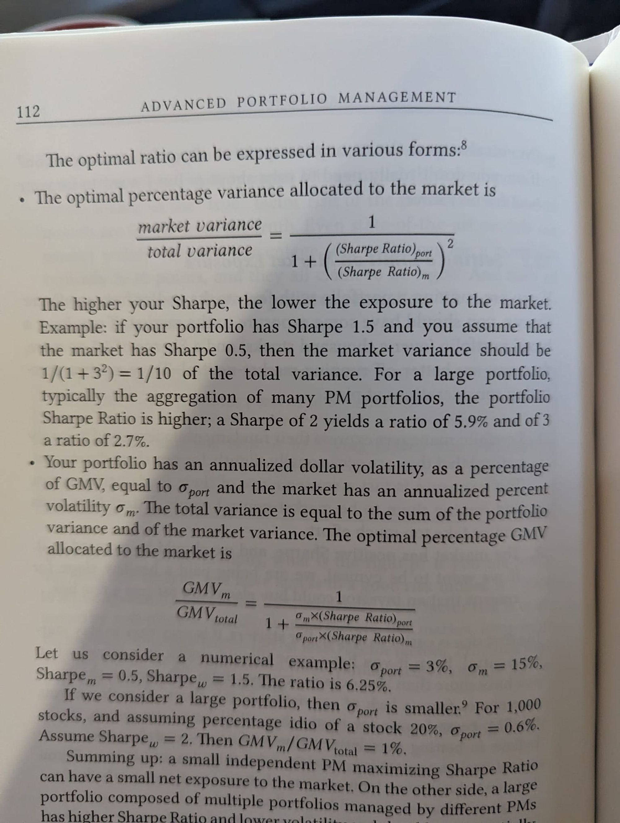
- Setting a limit on market exposure
- The higher your Sharpe ratio, the more market neutral you should be. Market exposure is a constraint on leverage.
- It can take too much effort or distort sizes to stay perfectly market neutral. Cynically, you are also being paid a healthy slope for returns that an investor would buy elsewhere for just a few basis points.
- In summary, a small independent portfolio manager (PM) maximizing Sharpe ratios can have a small net exposure to the market. On the other hand, a large portfolio composed of multiple portfolios managed by different PMs has higher Sharpe ratios and lower volatility, and should essentially run market neutral. The PMs contributing to this portfolio should also run market neutral.
- Setting an upper limit on single stock holdings
- 2 considerations:
- Liquidity
- The low signal to noise ratio in investment theses
- An intuitive Insight that falls out of the math: the larger the ratio between realized returns for high conviction stocks and low conviction stocks the more concentrated the portfolio can be. the author calls this the conviction profitability ratio. Be careful the error band around this measure is wide and in turn drives the range of possible single stock limits
- Systematic hedging in portfolio management
- automatic hedging program
- this is an optimization run at regular intervals (ie daily) to reduce factor risks
- Factor mimicking portfolios
- This is an internal facility that produces factors on demand. They are synthetic assets that mimic factor returns.
- Fully Automated Portfolio Construction
- The PM only inputs investment ideas, and the optimizer generates a portfolio that is efficiently traded and sized within factor risk limits.
3 approaches
Chapter 8: Understand your performance
The Earth rotates around the Sun at a speed of 67,000mph. When I go out for my occasional run, my own speed is in the tens of thousands of miles per hour Should I take credit for this amazing performance? I wouldn't be completely lying if I bragged about this with friends (which I do); but it would be more transparent if I mentioned that my speed record is in the frame reference of the Sun. In this frame of ref- erence, my speed is indistinguishable from Usain Bolt's. This factoid obscures the vast difference in skill between the two of us. To really understand the difference, we need to change the frame of reference. Another way to interpret the decomposition of returns is a method to change the frame of reference in investing. Total returns - and a portfolio's total PnL - live in the Sun's frame of reference. It is easy to fool ourselves with the belief that we beat birds, airplanes and supermen at their own game. Idiosyncratic returns and PnL live in the Earth's frame of reference. If we want to compare our performance to that of our peers, or to our very own past performance, we need to move to this frame. Factor-based performance attribution makes it possible.
Selection, Sizing, Timing
Decompose idiosyncratic PnL into:
- Selection: being directionally right
- Sizing: being right about the absolute value of returns
- Timing: taking risk when your theses are more correct than average
There is anecdotal evidence that PMs have at best very little timing skill, moderately-positive-to-moderately-negative sizing skill, and primarily selection skills. When you detect positive sizing or timing skill, you should treasure it and nurture it. When you don't, you can improve your performance by equalizing your positions within each date and/or across time.
Diversification has a cost
- Conceptually and mathematically diversification is not itself a skill but a skill multiplier.
- Diversification improves risk adjusted performance. P&l sums linearly while fluctuations average out.
- You don't need a high hitting probability to have great performance. If you're hitting, probability is 51% and the portfolio has 70 stocks. The information ratio is an excellent 2.6. This is why stat arb strategies can have such high risk adjusted performance. If you trade 3000 stocks to achieve an IR of 8, you only need a hitting probability of 50.5%
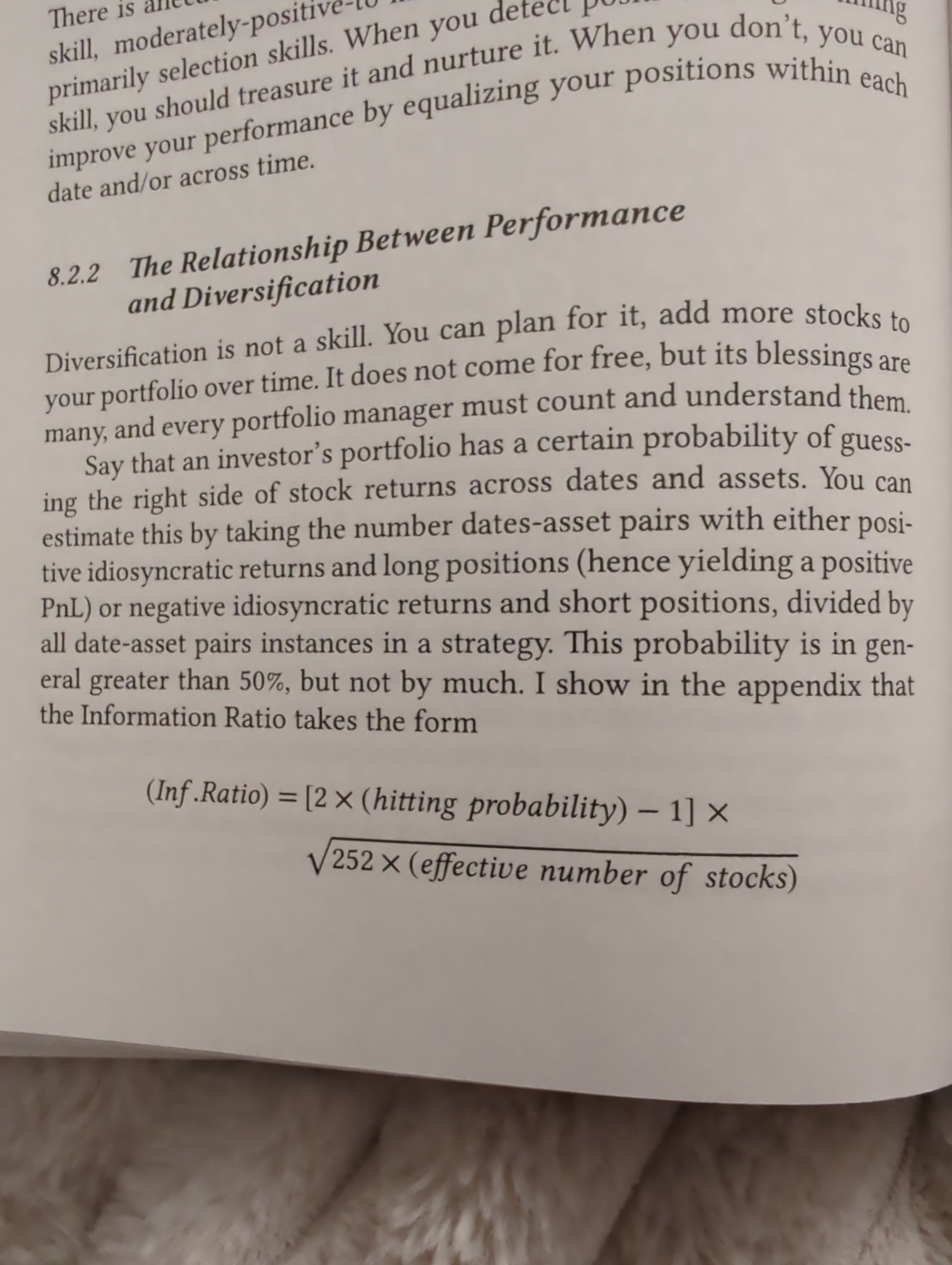
The formula contains 2 insights.
- The best increase in diversification comes when the signals on the breadth of the universe are not diluted (is adding more analysts vs splitting an existing analyst’s time). The cost shows up as a decline in information ratio because hit rate is inversely correlated with breadth past a certain point (limits of attention).
- In sum: having a broader portfolio is beneficial to risk adjusted performance and proportion to the square root of the effective number of stocks provided that the ability to forecast returns at the asset level is not negatively impacted.
Trading Events Efficiently
A manager can earn 25 to 50% of her PNL from earnings related bets. Therefore, it is important to develop a rational process for positioning and trading around earnings or at least to systematically think about the issue.
This section expounds on the quantitative reasoning behind the following heuristics:
1. Size at the event should be proportional to expected return;
2. Size at the event should be smaller if, everything else being equal. transaction costs are higher;
3. If the time from thesis formation to the event is shorter, everything else being equal, the size at the event should be smaller because there is less time to build it;
4. Following the event, the position should be exited, as it consumes the risk and capital budget of the PM.
Alternative Data
An example of using the existing factor model framework to put alternative data into production…the example uses Short Interest (heavily shorted stocks have historically underperformed lightly shorted stocks, although this anomaly has shrank since 2017)
1. Feature Generation: we covered this in 5.2. Features are borrow rate or short ratio. Sometimes we multiply short interest by a dummy variable representing the sector.
2. Feature Transformation: this step is sometimes omitted, in which case we just use the latest value of the short ratio. In the case of short interest, it is sometimes useful to consider the change vs. long-term average, e.g., current short interest against past three-month average.
3. Orthogonalization: this can be interpreted as a "cleaning stage": we regress the short interest features against the risk model loadings. Essentially, we try to "explain" short interest using the risk model, and then we keep the component that is not explained.
4. Cross-Sectional Regression: this step is the same as factor model estimation. The intuition behind this step is to check whether the short-interest loadings and the asset returns are correlated. If they are, then the short-interest return is not zero
5. Performance Metrics: Finally we explore the performance of short interest. Is the expected return non-zero? What is the Sharpe? Do loadings change all the time, so that they are hard to interpret or invest in?
Chapter 9: Manage Your Losses
- Stop loss rules hanging over a PM are a partial hedge against the PMs long call business proposition that otherwise prefers maximum volatility
- Stop-loss exists to ensure survival of a firm not to improve the performance of a strategy. There is a price to pay. We just need to make sure we are not overpaying or at least that we understand the trade-off between survivability and the parameters of stop-loss
- Stop-loss rules have two drawbacks:
- Transaction costs due to trading induced by de-grossing and re-grossing portfolios.
- Performance degradation due to forgone profits.
- Differences between the simple rule of single-threshold and two-threshold stop-loss are small.
- Performance degradation is a bigger concern than transaction costs. Choose the stop-loss threshold for your strategy or for PMs in your firm, based on trade-off curves in the chapters.
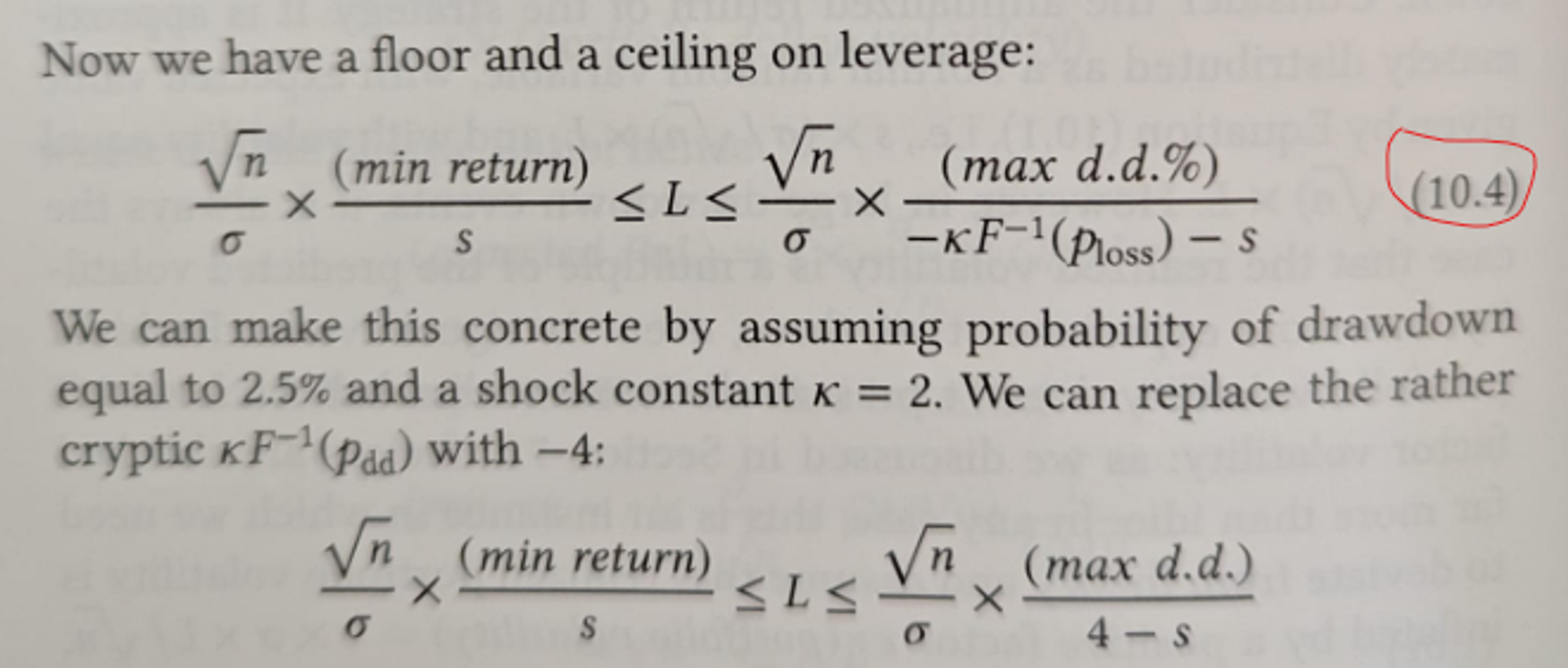
Chapter 10: Setting your leverage ratio
This chapter gives a framework for leverage decisions. Formulas produce minimum and maximum leverages.
Min leverage
Depends on the following variables:
- idio volatility
- number of stocks (breadth)
- sharpe ratio
- minimum required return
Intuitions based on the math:
- This produces a lower bound on leverage
- That lower bound is proportional to minimum return
- The higher the sharpe the lower the required leverage
Max leverage
Depends on the following variables:
- max drawdown allowable
- probability of max drawdown
- number of stocks
- sharpe ratio
- minimum required return
Intuitions based on the math:
- Maximum leverage is proportional to maximum drawdown
- A higher Sharpe ratio corresponds to a higher maximum leverage.
- It is possible that the lower bound on leverage is higher than the upper bound. This is a strategy which is not sustainable from a risk perspective — This is a potential explanation of “why so many hedge funds fail”
In sum:
- Target returns determine leverages lower bound; leverage is a return multiplier.
- Maximum acceptable loss determines leverages upper bound
- Breadth, volatility, and Sharpe ratio tie the two together.